Bayesian inference for state-space models
Defining a prior distribution
We have already seen that module particles.distributions defines various ProbDist objects; i.e. objects that represent probability distribution. Such objects have methods to simulate random variates, compute the log-density, and so on.
This module defines in particular a class called StructDist, whose methods take as inputs and outputs structured arrays. This is what we are going to use to define prior distributions. Here is a simple example:
[1]:
import warnings; warnings.simplefilter('ignore')  # hide warnings

from matplotlib import pyplot as plt
import numpy as np

from particles import distributions as dists

prior_dict = {'mu': dists.Normal(scale=2.),
              'rho': dists.Uniform(a=-1., b=1.),
              'sigma':dists.Gamma()}
my_prior = dists.StructDist(prior_dict)
Object my_prior represents a distribution for \(\theta=(\mu, \rho, \sigma)\) where \(\mu\sim N(0,2^2)\), \(\rho \sim \mathcal{U}([-1,1])\), \(\sigma \sim \mathrm{Gamma}(1, 1)\), independently. We may now sample from this distribution, or compute its pdf, and so on. For each of the operations, the inputs and outputs must be structured arrays, with named variables 'rho' and 'sigma'.
[2]:
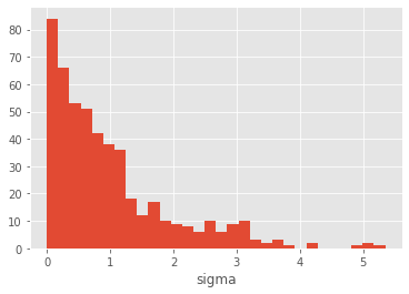
theta = my_prior.rvs(size=500)  # sample 500 theta-parameters

plt.style.use('ggplot')
plt.hist(theta['sigma'], 30);
plt.xlabel('sigma')

plt.figure()
z = my_prior.logpdf(theta)
plt.hist(z, 30)
plt.xlabel('log-pdf');
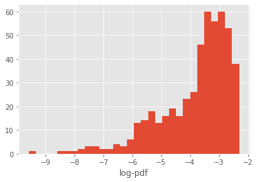
We may want to transform sigma into its logarithm, so that the support of the distribution is not constrained to \(\mathbb{R}^+\):
[3]:
another_prior_dict = {'rho': dists.Uniform(a=-1., b=1.),
                      'log_sigma':dists.LogD(dists.Gamma())}
another_prior = dists.StructDist(another_prior_dict)
another_theta = another_prior.rvs(size=100)

plt.hist(another_theta['log_sigma'], 20)
plt.xlabel('log-sigma');
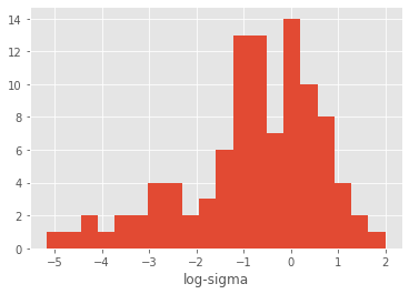
Now, another_theta contains two variables, rho and log_sigma, and the latter variable is distributed according to \(Y=\log(X)\), with \(X\sim \mathrm{Gamma}(1, 1)\). (The documentation of module distributions has more details on transformed distributions.)
We may also want to introduce dependencies between \(\rho\) and \(\sigma\). Consider this:
[4]:
from collections import OrderedDict

dep_prior_dict = OrderedDict()
dep_prior_dict['rho'] = dists.Uniform(a=0., b=1.)
dep_prior_dict['sigma'] = dists.Cond( lambda theta: dists.Gamma(b=1./theta['rho']))
dep_prior = dists.StructDist(dep_prior_dict)
dep_theta = dep_prior.rvs(size=2000)

plt.scatter(dep_theta['rho'], dep_theta['sigma'])
plt.axis([0., 1., 0., 8.])
plt.xlabel('rho')
plt.ylabel('sigma');
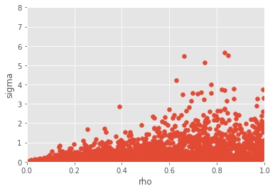
The lines above encodes a chain rule decomposition: first we specify the marginal distribution of \(\rho\), then we specify the distribution of \(\sigma\) given \(\rho\). A standard dictionary in Python is unordered: there is no way to make sure that the keys appear in a certain order. Thus we use instead an OrderedDict, and define first the distribution of \(\rho\), then the distribution of \(\sigma\) given \(\rho\); Cond is a particular ProbDist class
that defines a conditional distribution, based on a function that takes an argument theta, and returns a ProbDist object.
All the example above involve univariate distributions; however, the components of StructDist also accept multivariate distributions.
[5]:
reg_prior_dict = OrderedDict()
reg_prior_dict['sigma2'] = dists.InvGamma(a=2., b=3.)
reg_prior_dict['beta'] = dists.MvNormal(cov=np.eye(20))
reg_prior = dists.StructDist(reg_prior_dict)
reg_theta = reg_prior.rvs(size=200)
Bayesian inference for state-space models
We return to the simplified stochastic volatility introduced in the basic tutorial:
\begin{align*} X_0 & \sim N\left(\mu, \frac{\sigma^2}{1-\rho^2}\right) \\ X_t|X_{t-1}=x_{t-1} & \sim N\left( \mu + \rho (x_{t-1}-\mu), \sigma^2\right) \\ Y_t|X_t=x_t & \sim N\left(0, e^{x_t}\right) \end{align*}
which we implemented as follows (this time with default values for the parameters):
[6]:
from particles import state_space_models as ssm

class StochVol(ssm.StateSpaceModel):
    default_parameters = {'mu':-1., 'rho':0.95, 'sigma': 0.2}
    def PX0(self):  # Distribution of X_0
        return dists.Normal(loc=self.mu, scale=self.sigma / np.sqrt(1. - self.rho**2))
    def PX(self, t, xp):  # Distribution of X_t given X_{t-1}=xp (p=past)
        return dists.Normal(loc=self.mu + self.rho * (xp - self.mu), scale=self.sigma)
    def PY(self, t, xp, x):  # Distribution of Y_t given X_t=x (and possibly X_{t-1}=xp)
        return dists.Normal(loc=0., scale=np.exp(x))
We mentioned in the basic tutorial that StochVol represents the parameteric class of univariate stochastic volatility model. Indeed, StochVol will be the object we pass to Bayesian inference algorithms (such as PMMH or SMC\(^2\)) in order to perform inference with respect to that class of models.
PMMH (Particle marginal Metropolis-Hastings)
Let’s try first PMMH. This is a Metropolis-Hastings algorithm that samples from the posterior of parameter \(\theta\) (given the data). However, since the corresponding likelihood is intractable, each iteration of PMMH runs a particle filter that approximates it.
[9]:
from particles import mcmc
from particles import datasets as dts  # real datasets available in the package

# real data
T = 50
data = dts.GBP_vs_USD_9798().data[:T]

my_pmmh = mcmc.PMMH(ssm_cls=StochVol, prior=my_prior, data=data, Nx=200,
                    niter=1000)
my_pmmh.run();  # may take several seconds...
The arguments we set when instantiating class PMMH requires little explanation; just in case:
Nxis the number of particles (for the particle filter run at each iteration);niteris the number of MCMC iterations.
Upon completion, object my_pmmh.chain is a ThetaParticles object, with the following attributes:
my_pmmh.chain.thetais a structured array of size 10 (the number of iterations) with keys'mu','rho'and'sigma';my_pmmh.chain.lpostis an array of length 10, contanining the (estimated) log-posterior density for each simulated \(\theta\).
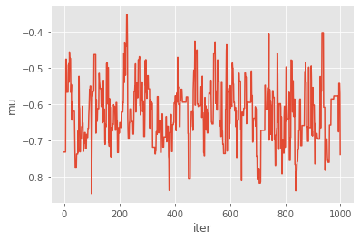
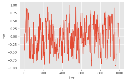
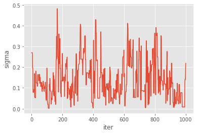
Let’s plot the mcmc traces.
[10]:
for p in prior_dict.keys():  # loop over mu, theta, rho
    plt.figure()
    plt.plot(my_pmmh.chain.theta[p])
    plt.xlabel('iter')
    plt.ylabel(p)
You might wonder what type of Metropolis sampler is really implemented here:
the starting point of the chain is sampled from the prior; you may instead set it to a specific value using option
starting_point(when instantiatingPMMH);the proposal is an adaptative Gaussian random walk: this means that the covariance matrix of the random step is calibrated on the fly on past simulations (using vanishing adaptation). This may be disabled by setting option
adaptive=False;a bootstrap filter is run to approximate the log-likelihood; you may use a different filter (e.g. a guided filter) by passing a
FeynmanKacclass to optionfk_cls;you may also want to pass various parameters to each call to
SMCthrough (dict) argumentsmc_options; e.g.smc_options={'qmc': True}will make each particle filter a SQMC algorithm.
Thus, by and large, quite a lot of flexibility is hidden behind this default behaviour.
Particle Gibbs
PMMH is just a particular instance of the general family of PMCMC samplers; that is MCMC samplers that run some particle filter at each iteration. Another instance is Particle Gibbs (PG), where one simulate alternatively: 1. from the distribution of \(\theta\) given the states and the data; 2. renew the state trajectory through a CSMC (conditional SMC step).
Since Step 1 is model- (and user-)dependent, you need to define it for the model you are considering. This is done by sub-classing ParticleGibbs and defining method update_theta as follows:
[11]:
class PGStochVol(mcmc.ParticleGibbs):
    def update_theta(self, theta, x):
        new_theta = theta.copy()
        sigma, rho = 0.2, 0.95  # fixed values
        xlag = np.array(x[1:] + [0.,])
        dx = (x - rho * xlag) / (1. - rho)
        s = sigma / (1. - rho)**2
        new_theta['mu'] = self.prior.laws['mu'].posterior(dx, sigma=s).rvs()
        return new_theta
For simplicity \(\rho\) and \(\sigma\) are kept constant; only \(\mu\) is updated. This means we are actually sampling from the posterior of \(\mu\) given the data, while these other parameters are kept constant. Let’s run our PG algorithm:
[12]:
pg = PGStochVol(ssm_cls=StochVol, data=data, prior=my_prior, Nx=200, niter=1000)
pg.run()  # may take several seconds...
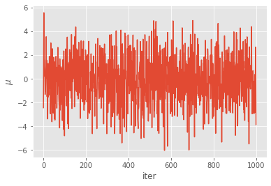
Now let’s plot the results:
[16]:
plt.plot(pg.chain.theta['mu'])
plt.xlabel('iter')
plt.ylabel(r'$\mu$')
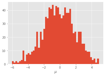
plt.figure()
plt.hist(pg.chain.theta['mu'][20:], 50)
plt.xlabel(r'$\mu$');
SMC^2
Finally, we consider SMC\(^2\), a SMC algorithm that makes it possible to approximate:
all the partial posteriors (of \(\theta\) given \(y_{0:t}\), for \(t=0, 1, ..., T\)) rather than only the final posterior;
the marginal likelihoods of the data.
SMC\(^2\) is a two-level SMC sampler:
it simulates many \(\theta\)-values from the prior, and update their weights recursively, according to the likelihood of each new datapoint;
however, since these likelihood factors are intractable, for each \(\theta\), a particle filter is run to approximate it; hence a number \(N_x\) of \(x\)-particles are generated for, and attached to, each \(\theta\).
The class SMC2 is defined inside module smc_samplers. It is run in the same way as the other SMC algorithms.
[17]:
import particles
from particles import smc_samplers as ssp

fk_smc2 = ssp.SMC2(ssm_cls=StochVol, data=data, prior=my_prior,init_Nx=50,
                   ar_to_increase_Nx=0.1)
alg_smc2 = particles.SMC(fk=fk_smc2, N=500)
alg_smc2.run()
Again, a few choices are made for you by default:
A bootstrap filter is run for each \(\theta-\)particle; this may be changed by setting option
fk_classwhile instantiatingSMC2; e.g.fk_class=ssm.GuidedPFwill run instead a guided filter.Option
init_Nxdetermines the initial number of \(x-\)particles; the algorithm automatically increases \(N_x\) each time the acceptance rate drops below \(10\%\) (as specified through optionar_to_increase=0.1. Set this this option to0.if you do not want to increase \(N_x\) in the course of t he algorithm.The particle filters (in the \(x-\)dimension) are run with the default options of class
SMC; e.g. resampling is set tosystematicand so on; other options may be set by using optionsmc_options.
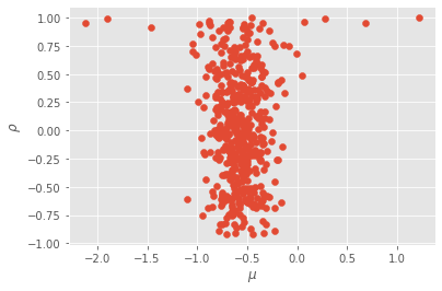
[19]:
plt.scatter(alg_smc2.X.theta['mu'], alg_smc2.X.theta['rho'])
plt.xlabel(r'$\mu$')
plt.ylabel(r'$\rho$');