Advanced Tutorial (geared toward state-space models)
This tutorial covers more or less the same topics as the basic tutorial (filtering and smoothing of state-space models), but in greater detail.
Defining state-space models
We consider a state-space model of the form:
\begin{align*} X_0 & \sim N(0, 1) \\ X_t & = f(X_{t-1}) + U_t, \quad U_t \sim N(0, \sigma_X^2) \\ Y_t & = X_t + V_t, \quad V_t \sim N(0, \sigma_Y^2) \end{align*}
where function \(f\) is defined as follows: \(f(x) = x + \tau_0 - \tau_1 * \exp( \tau_2 * x)\). This model comes from Population Ecology; there \(X_t\) stands for the logarithm of the population size of a given species. This model may be defined as follows.
[1]:
# the usual imports
from matplotlib import pyplot as plt
import seaborn as sb
import numpy as np

# imports from the package
import particles
from particles import state_space_models as ssm
from particles import distributions as dists


class ThetaLogistic(ssm.StateSpaceModel):
    """ Theta-Logistic state-space model (used in Ecology).
    """
    default_params = {'tau0':.15, 'tau1':.12, 'tau2':.1, 'sigmaX': 0.47, 'sigmaY': 0.39}

    def PX0(self):  # Distribution of X_0
        return dists.Normal()

    def f(self, x):
        return (x + self.tau0 - self.tau1 * np.exp(self.tau2 * x))

    def PX(self, t, xp):  #  Distribution of X_t given X_{t-1} = xp (p=past)
        return dists.Normal(loc=self.f(xp), scale=self.sigmaX)

    def PY(self, t, xp, x):  # Distribution of Y_t given X_t=x, and X_{t-1}=xp
        return dists.Normal(loc=x, scale=self.sigmaY)
This is most similar to what we did in the previous tutorial (for stochastic volatility models): methods PX0, PX and PY return objects defined in module distributions. (See the documentation of that module for a list of available distributions).
The only novelty is that we defined (as a class attribute) the dictionary default_parameters, which provides default values for each parameter. When it is defined, each parameter that is not set explicitly when instantiating (calling) ThetaLogistic is replaced by its default value:
[2]:
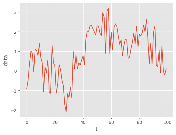
my_ssm = ThetaLogistic()  # use default values for all parameters
x, y = my_ssm.simulate(100)

plt.style.use('ggplot')
plt.plot(y)
plt.xlabel('t')
plt.ylabel('data');
“Bogus Parameters” (parameters that do not appear in PX0, PX and PY) are simply ignored:
[3]:
just_for_fun = ThetaLogistic(tau2=0.3, bogus=92.) # ok
This behaviour may look surprising, but it will allow us to define prior distributions that involve hyper-parameters.
Automatic definition of FeynmanKac objects
We have seen in the previous tutorial how to run a bootstrap filter: we first define some Bootstrap object, and then passes it to SMC.
[4]:
fk_boot = ssm.Bootstrap(ssm=my_ssm, data=y)
my_alg = particles.SMC(fk=fk_boot, N=100)
my_alg.run()
In fact, ssm.Bootstrap is a subclass of FeynmanKac, the base class for objects that represent “Feynman-Kac models” (covered in Chapters 5 and 10 of the book). To make things simple, a Feynman-Kac model is a “recipe” for our SMC algorithms; in particular, it tells us:
how to sample each particle \(X_t^n\) at time \(t\), given their ancestors \(X_{t-1}^n\);
how to reweight each particle \(X_t^n\) at time \(t\).
The bootstrap filter is a particular “recipe”, where:
we sample the particles \(X_t^n\) according to the state transition of the model; in our case a \(N(f(x_{t-1}),\sigma_X^2)\) distribution.
we reweight the particles according to the likelihood of the model; here the density of \(N(x_t,\sigma_Y^2)\) at point \(y_t\).
The class ssm.Bootstrap defines this recipe automatically from the supplied state-space model and data.
The bootstrap filter is not the only available “recipe”. We may want to run a guided filter, where the particles are simulated according to user-chosen proposal kernels. Such proposal kernels may be defined by adding methods proposal and proposal0 to our StateSpaceModel class:
[5]:
class ThetaLogistic_with_prop(ThetaLogistic):
    def proposal0(self, data):
        return self.PX0()
    def proposal(self, t, xp, data):
        prec_prior = 1. / self.sigmaX**2
        prec_lik = 1. / self.sigmaY**2
        var = 1. / (prec_prior + prec_lik)
        mu = var * (prec_prior * self.f(xp) + prec_lik * data[t])
        return dists.Normal(loc=mu, scale=np.sqrt(var))

my_better_ssm = ThetaLogistic_with_prop()
In this particular case, we implemented the “optimal” proposal, that is, the distribution of \(X_t\) given \(X_{t-1}\) and \(Y_t\). (Check this is indeed this case, this is a simple exercise!). (For simplicity, the proposal at time 0 is simply the distribution of X_0, so this one is not optimal.)
Now we may define our guided Feynman-Kac model:
[6]:
fk_guided = ssm.GuidedPF(ssm=my_better_ssm, data=y)
An APF (auxiliarly particle filter) may be implemented in the same way: for this, we must also define method logeta, which computes the auxiliary function used in the resampling step; see the documentation and the end of Chapter 10 of the book.
Running a particle filter
Here is the signature of class SMC:
[7]:
alg = particles.SMC(fk=fk_guided, N=100, qmc=False, resampling='systematic', ESSrmin=0.5,
                    store_history=False, verbose=False, collect=None)
Apart from fk (which expects a FeynmanKac object), all the other arguments are optional. Here is what they do:
N: the number of particlesqmc: whether to use the QMC (quasi-Monte Carlo) versionresampling: which resampling scheme to use (possible choices:'multinomial','residual','stratified','systematic'and'ssp')ESSrmin: the particle filter resamples at each iteration such that ESS / N is below this threshold; set it to1.(resp.0.) to resample every time (resp. to never resample)verbose: whether to print progress information
The remaining arguments (store_history and collect) will be explained in the following sections.
Once we have a created a SMC object, we may run it, either step by step, or in one go. For instance:
[8]:
next(alg) # processes data-point y_0
next(alg)  # processes data-point y_1
for _ in range(8):
    next(alg)  # processes data-points y_3 to y_9
# alg.run()  # would process all the remaining data-points
At any time, object alg has the following attributes:
alg.t: index of next iterationalg.X: the N current particles \(X_t^n\); typically a (N,) or (N,d) numpy arrayalg.W: the N normalised weights \(W_t^n\) (a (N,) numpy array)alg.Xp: the N particles at the previous iteration, \(X_{t-1}^n\)alg.A: the N ancestor variables: A[3] = 12 means that the parent of \(X_t^3\) was \(X_{t-1}^{12}\).alg.summaries: various summaries collected at each iteration.
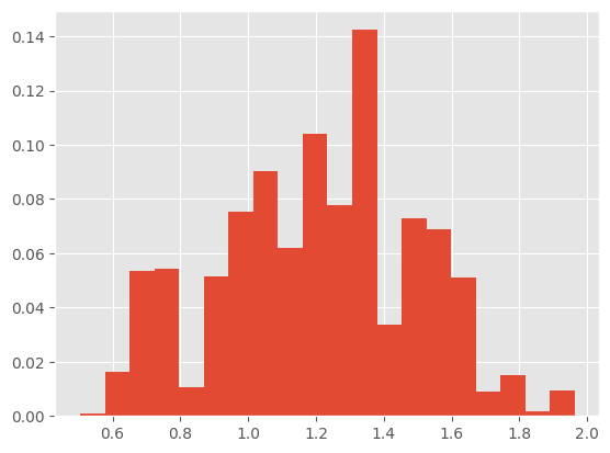
Let’s do for instance a weighted histogram of the particles.
[9]:
plt.hist(alg.X, 20, weights=alg.W);
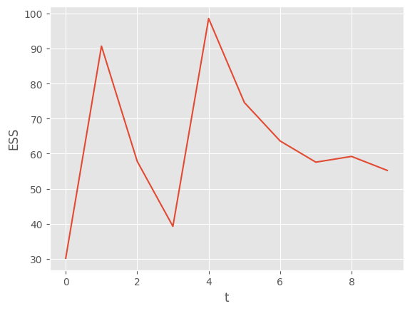
Object alg.summaries contains various lists of quantities collected at each iteration, such as:
* `alg.summaries.ESSs`: the ESS (effective sample size) at each iteration
* `alg.summaries.rs_flags`: whether or not resampling was triggered at each step
* `alg.summaries.logLts`: estimates of the log-likelihood of the data $y_{0:t}$
All this and more is explained in the documentation of the collectors module. Let’s plot the ESS and the log-likelihood:
[10]:
plt.plot(alg.summaries.ESSs)
plt.xlabel('t')
plt.ylabel('ESS');
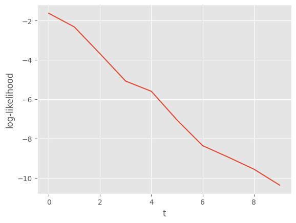
[11]:
plt.plot(alg.summaries.logLts)
plt.xlabel('t')
plt.ylabel('log-likelihood');
Running many particle filters in one go
Function multiSMC accepts the same arguments as SMC plus the following extra arguments:
nruns: number of runsnprocs: if >0, number of CPU cores to use; if <=0, number of cores not to use; i.e.nprocs=0means use all coresout_func: a function that is applied to each resulting particle filter (see below).
To explain how exactly multiSMC works, let’s try to compare the bootstrap and guided filters for the theta-logistic model we defined at the beginning of this tutorial:
[12]:
outf = lambda pf: pf.logLt
results = particles.multiSMC(fk={'boot':fk_boot, 'guid':fk_guided},
                             nruns=20, nprocs=1, out_func=outf)
The command above runs 40 particle algorithms (on a single core): 20 bootstrap filters, and 20 guided filters. The output, results, is a list of 40 dictionaries; each dictionary contains the following (key, value) pairs:
'model': either'boot'or'guid'(according to whether a bootstrap or guided filter has been run)'run': a run indicator (between 0 and 19)'output': the result ofoutf(pf)where pf is the SMC object that was run. (Ifoutfis set to None, then the SMC object is returned.)
The rationale for function outf is that SMC objects may take a lot of memory in certain cases (especially if you set store_history=True, see section on smoothing below), so we may want to save only some results of interest rather than the complete object itself. Here the output is simply the estimate of the log-likelihood of the (complete) data computed by each particle filter. Let’s check if the guided filter provides lower-variance estimates, relative to the bootstrap filter.
[13]:
sb.boxplot(x=[r['fk'] for r in results], y=[r['output'] for r in results])
[13]:
<Axes: >
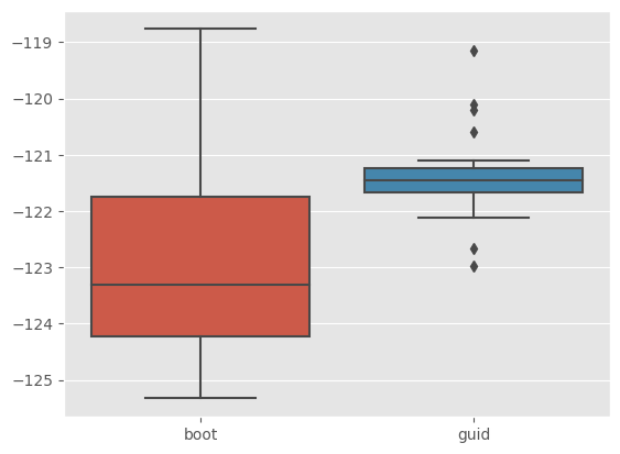
This is indeed the case. To understand this line of code, you must be a bit familiar with list comprehensions.
More generally, function multiSMC may be used to run multiple SMC algorithms, while varying any possible arguments; for more details, see the documentation of multiSMC and of the module particles.utils.
Collectors, on-line smoothing
We have said that alg.summaries (where alg is a SMC object) contains lists that contains quantities computed each iteration (such as the ESS, the log-likelihood estimates). It is possible to compute extra such quantities such as:
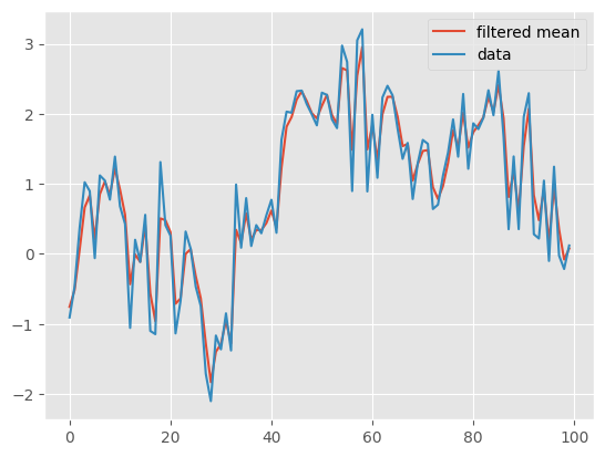
moments: at each time \(t\), a dictionary with keys ‘mean’, and ‘var’, which stores the component-wise weighted means and variances.
on-line smoothing estimates (naive, and \(O(N^2)\), see module
collectorsfor more details)
by providing a list of Collector objects to parameter collect. For instance, to collect moments:
[14]:
from particles.collectors import Moments

alg_with_mom = particles.SMC(fk=fk_guided, N=100, collect=[Moments()])
alg_with_mom.run()

plt.plot([m['mean'] for m in alg_with_mom.summaries.moments],
         label='filtered mean')
plt.plot(y, label='data')
plt.legend()
[14]:
<matplotlib.legend.Legend at 0x7ff95979a050>
Off-line smoothing
Off-line smoothing is the task of approximating, at some final time \(T\) (i.e. when we have stopped acquiring data), the distribution of all the states, \(X_{0:T}\), given the full data, \(Y_{0:T}\).
To run a particular off-line smoothing algorithm, one must first run a particle filter, and save its history:
[15]:
alg = particles.SMC(fk=fk_guided, N=100, store_history=True)
alg.run()
Now alg has a hist attribute, which is a ParticleHistory object. Basically, alg.hist recorded, at each time \(t\):
the N particles \(X_t^n\)
their weights \(W_t^n\)
the N ancestor variables
Smoothing algorithms are implemented as methods of class ParticleHistory. For instance, the FFBS (forward filtering backward sampling) algorithm, which samples complete smoothing trajectories, may be called as follows:
[18]:
trajectories = alg.hist.backward_sampling_ON2(5)
plt.plot(trajectories);
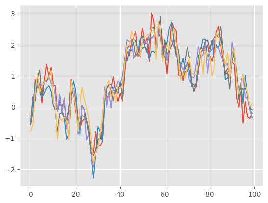
The output of backward_sampling_ON2 is a list of 100 arrays: trajectories[t][m] is the \(t\)-component of trajectory \(m\). (If you want to turn it into a numpy array, simply do: np.array(trajectories).)
Remark: particles implement several FFBS algorithms; backward_sampling_ON2 implements the most basic one, which has complexity \(\mathcal{O}(N^2)\) if you want to generate \(N\) trajectories (where \(N\) is the initial number of particles). There are faster variants, the recommended one, based on Dau & Chopin (2023), is backward_sampling_mcmc, which relies on MCMC. This is fast, and has a deterministic running time, \(\mathcal{O}(N)\), contrary to some other
rejection-based schemes (which are also implemented). To learn more about this, see again Dau & Chopin (2023).
Remark: Two-filter smoothing is also available. The difficulty with two-filter smoothing is that it requires to design an “information filter”, that is a particle filter that computes recursively (backwards) the likelihood of the model. Since this is not trivial for the model considered here, we refer to Section 12.5 of the book and the documentation of package smoothing.