Manual definition of Feynman-Kac models

It is not particularly difficult to define manually your own FeynmanKac classes. Consider the following problem: we would like to approximate the probability that \(X_t \in [a,b]\) for all \(0\leq t < T\), where \((X_t)\) is a random walk: \(X_0\sim N(0,1)\), and

\[X_t | X_{t-1} = x_{t-1} \sim N(x_{t-1}, 1).\]

This probability, at time \(t\), equals \(L_t\), the normalising constant of the following Feynman-Kac sequence of distributions:

\begin{equation} \mathbb{Q}_t(dx_{0:t}) = \frac{1}{L_t} M_0(dx_0)\prod_{s=1}^t M_s(x_{s-1},dx_s) \prod_{s=0}^t G_s(x_{s-1}, x_s) \end{equation}

where:

• \(M_0(dx_0)\) is the \(N(0,1)\) distribution;

• \(M_s(x_{s-1},dx_s)\) is the \(N(x_{s-1}, 1)\) distribution;

• \(G_s(x_{s-1}, x_s)= \mathbb{1}_{[0,\epsilon]}(x_s)\)

Let’s define the corresponding FeymanKac object:

from matplotlib import pyplot as plt
import seaborn as sb
import numpy as np
from scipy import stats

import particles

class GaussianProb(particles.FeynmanKac):
    def __init__(self, a=0., b=1., T=10):
        self.a, self.b, self.T = a, b, T

    def M0(self, N):
        return stats.norm.rvs(size=N)

    def M(self, t, xp):
        return stats.norm.rvs(loc=xp, size=xp.shape)

    def logG(self, t, xp, x):
        return np.where((x < self.b) & (x > self.a), 0., -np.inf)

The class above defines:

• the initial distribution, \(M_0(dx_0)\) and the kernels \(M_t(x_{t-1}, dx_t)\), through methods M0(self, N) and M(self, t, xp). In fact, these methods simulate \(N\) random variables from the corresponding distributions.

• Function logG(self, t, xp, x) returns the log of function \(G_t(x_{t-1}, x_t)\).

Methods M0 and M also define implicitly how the \(N\) particles should be represented internally: as a (N,) numpy array. Indeed, at time \(0\), method M0 generates a (N,) numpy array, and at times \(t\geq 1\), method M takes as an input (xp) and returns as an output arrays of shape (N,). We could use another type of object to represent our \(N\) particles; for instance, the smc_samplers module defines a ThetaParticles class for storing \(N\) particles representing \(N\) parameter values (and associated information).

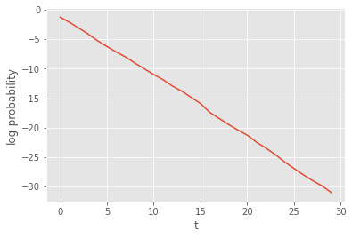
Now let’s run the corresponding SMC algorithm:

fk_gp = GaussianProb(a=0., b=1., T=30)
alg = particles.SMC(fk=fk_gp, N=100)
alg.run()

plt.style.use('ggplot')
plt.plot(alg.summaries.logLts)
plt.xlabel('t')
plt.ylabel(r'log-probability');

That was not so hard. However our implementation suffers from several limitations:

1. The SMC sampler we ran may be quite inefficient when interval \([a,b]\) is small; in that case many particles should get a zero weight at each iteration.

2. We cannot currently run the SQMC algorithm (the quasi Monte Carlo version of SMC); to do so, we need to specify the Markov kernels \(M_t\) in a different way: not as simulators, but as deterministic functions that take as inputs uniform variates (see below).

Let’s address the second point:

class GaussianProb(particles.FeynmanKac):
    du = 1  # dimension of uniform variates

    def __init__(self, a=0., b=1., T=10):
        self.a, self.b, self.T = a, b, T

    def M0(self, N):
        return stats.norm.rvs(size=N)

    def M(self, t, xp):
        return stats.norm.rvs(loc=xp, size=xp.shape)

    def Gamma0(self, u):
        return stats.norm.ppf(u)

    def Gamma(self, t, xp, u):
        return stats.norm.ppf(u, loc=xp)

    def logG(self, t, xp, x):
        return np.where((x < self.b) & (x > self.a), 0., -np.inf)

fk_gp = GaussianProb(a=0., b=1., T=30)

We have added:

• methods Gamma0 and Gamma, which define the deterministic functions \(\Gamma_0\) and \(\Gamma\) we mentioned above. Mathematically, for \(U\sim \mathcal{U}([0,1]^{d_u})\), then \(\Gamma_0(U)\) is distributed according to \(M_0(dx_0)\), and \(\Gamma_t(x_{t-1}, U)\) is distributed according to \(M_t(x_{t-1}, dx_t)\).

• class attribute du, i.e. \(d_u\), the dimension of the \(u\)-argument of functions \(\Gamma_0\) and \(\Gamma_t\).

We are now able to run both the SMC and the SQMC algorithms that corresponds to the Feyman-Kac model of interest; let’s compare their respective performance. (Recall that function multiSMC runs several algorithms multiple times, possibly with varying parameters; here we vary parameter qmc, which determines whether we run SMC or SMQC.)

results = particles.multiSMC(fk=fk_gp, qmc={'smc': False, 'sqmc': True}, N=100, nruns=10)

sb.boxplot(x=[r['qmc'] for r in results], y=[r['output'].logLt for r in results]);

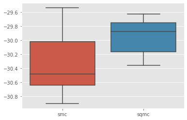
We do get some variance reduction, but not so much. Let’s see if we can do better by addressing point 1 above.

The considered problem has the structure of a state-space model, where process \((X_t)\) is a random walk, \(Y_t = \mathbb{1}_{[a,b]}(X_t)\), and \(y_t=1\) for all \(t\)’s. This remark leads us to define alternative Feynman-Kac models, that would correspond to guided and auxiliary formalisms of that state-space model. In particular, for the guided filter, the optimal proposal distribution, i.e. the distribution of \(X_t|X_{t-1}, Y_t\), is simply a Gaussian distribution truncated to interval \([a, b]\); let’s implement the corresponding Feynman-Kac class.

def logprobint(a, b, x):
    """ returns log probability that X_t\in[a,b] conditional on X_{t-1}=x
    """
    return np.log(stats.norm.cdf(b - x) - stats.norm.cdf(a - x))

class Guided_GP(GaussianProb):

    def Gamma(self, t, xp, u):
        au = stats.norm.cdf(self.a - xp)
        bu = stats.norm.cdf(self.b - xp)
        return xp + stats.norm.ppf(au + u * (bu - au))

    def Gamma0(self, u):
        return self.Gamma(0, 0., u)

    def M(self, t, xp):
        return self.Gamma(t, xp, stats.uniform.rvs(size=xp.shape))

    def M0(self, N):
        return self.Gamma0(stats.uniform.rvs(size=N))

    def logG(self, t, xp, x):
        if t == 0:
            return np.full(x.shape, logprobint(self.a, self.b, 0.))
        else:
            return logprobint(self.a, self.b, xp)

fk_guided = Guided_GP(a=0., b=1., T=30)

In this particular case, it is a bit more convenient to define methods Gamma0 and Gamma first, and then define methods M0 and M.

To derive the APF version, we must define the auxiliary functions (functions \(\eta_t\) in Chapter 10 of the book) that modify the resampling probabilities; in practice, we define the log of these functions, as follows:

class APF_GP(Guided_GP):
    def logeta(self, t, x):
        return logprobint(self.a, self.b, x)

fk_apf = APF_GP(a=0., b=1., T=30)

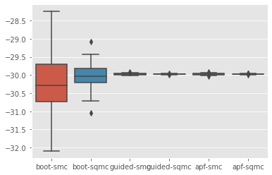
Ok, now everything is set! We can do a 3x2 comparison of SMC versus SQMC, for the 3 considered Feynman-Kac models.

results = particles.multiSMC(fk={'boot':fk_gp, 'guided':fk_guided, 'apf': fk_apf},
                             N=100, qmc={'smc': False, 'sqmc': True}, nruns=200)

sb.boxplot(x=['%s-%s'%(r['fk'], r['qmc'])  for r in results], y=[r['output'].logLt for r in results]);

Let’s discard the bootstrap algorithms to better visualise the results for the other algorithms:

res_noboot = [r for r in results if r['fk']!='boot']
sb.boxplot(x=['%s-%s'%(r['fk'], r['qmc'])  for r in res_noboot], y=[r['output'].logLt for r in res_noboot]);

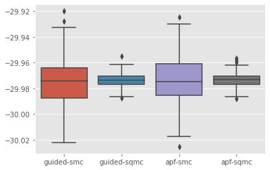
Voilà!