Basic tutorial

This basic tutorial gives a brief overview of some of functionality of the particles package. Details are deferred to more advanced tutorials.

First steps: defining a state-space model

We start by importing some standard libraries, plus some modules from the package.

%matplotlib inline
import warnings; warnings.simplefilter('ignore')  # hide warnings

# standard libraries
from matplotlib import pyplot as plt
import numpy as np
import seaborn as sb

# modules from particles
import particles  # core module
from particles import distributions as dists  # where probability distributions are defined
from particles import state_space_models as ssm  # where state-space models are defined
from particles.collectors import Moments

Let’s define our first state-space model class. We consider a basic stochastic volalitility model, that is: \begin{align*} X_0 & \sim N\left(\mu, \frac{\sigma^2}{1-\rho^2}\right), &\\ X_t|X_{t-1}=x_{t-1} & \sim N\left( \mu + \rho (x_{t-1}-\mu), \sigma^2\right), &\quad t\geq 1, \\ Y_t|X_t=x_t & \sim N\left(0, e^{x_t}\right),& \quad t\geq 0. \end{align*}

Note that this model depends on fixed parameter \(\theta=(\mu, \rho, \sigma)\).

In case you are not familiar with the notations above: a state-space model is a model for a joint process \((X_t, Y_t)\), where \((X_t)\) is an unobserved Markov process (the state of the system), and \(Y_t\) is some noisy measurement of \(X_t\) (hence it is observed). For instance, in stochastic volatility, \(Y_t\) is typically the log-return of some asset, and \(X_t\) its (unobserved) volatility.

The code below is hopefully transparent.

class StochVol(ssm.StateSpaceModel):
    def PX0(self):  # Distribution of X_0
        return dists.Normal(loc=self.mu, scale=self.sigma / np.sqrt(1. - self.rho**2))
    def PX(self, t, xp):  # Distribution of X_t given X_{t-1}=xp (p=past)
        return dists.Normal(loc=self.mu + self.rho * (xp - self.mu), scale=self.sigma)
    def PY(self, t, xp, x):  # Distribution of Y_t given X_t=x (and possibly X_{t-1}=xp)
        return dists.Normal(loc=0., scale=np.exp(x))

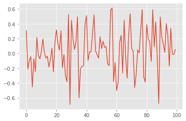
my_model = StochVol(mu=-1., rho=.9, sigma=.1)  # actual model
true_states, data = my_model.simulate(100)  # we simulate from the model 100 data points

plt.style.use('ggplot')
plt.figure()
plt.plot(data)

[<matplotlib.lines.Line2D at 0x7f602e517ca0>]

Methods PX0, PX and PY return objects that represent probability distributions (defined in module distributions. Parameters \(\mu\), \(\rho\) and \(\sigma\) are defined as attributes of a class instance: i.e. self.mu and so on. (self is the generic name for an instance of a class in Python.)

If your are not very familiar with OOP (object oriented programming) and related concepts (classes, instances, etc.), here is a simple way to understand them in our context:

• The class StochVol represents the parametric class of stochastic volatility models.

• The object my_model (a class instance of StochVol) defines a particular model, where parameters \(\mu\), \(\rho\) and \(\sigma\) are fixed to certain values.

In particular, we can inspect the attributes of my_model that store the parameter values.

my_model.mu, my_model.rho, my_model.sigma

(-1.0, 0.9, 0.1)

Class StochVol is a sub-class of StateSpaceModel. (You can see that from the first line of its definition.) For instance, it inherits a method called simulate that generates states and datapoints from the considered model.

Particle filtering

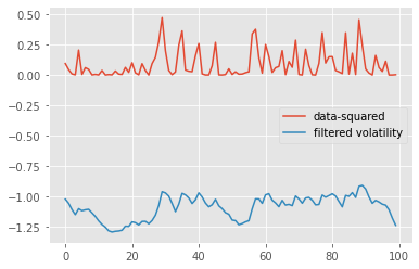
There are several particle algorithms that one may associate to a given state-space model. Here we consider the simplest option: the bootstrap filter. (See next tutorial for how to implement a guided or auxiliary filter.) The code below runs such a bootstrap filter for \(N=100\) particles, using stratified resampling.

fk_model = ssm.Bootstrap(ssm=my_model, data=data)  # we use the Bootstrap filter
pf = particles.SMC(fk=fk_model, N=100, resampling='stratified',
                   collect=[Moments()], store_history=True)  # the algorithm
pf.run()  # actual computation

# plot
plt.figure()
plt.plot([yt**2 for yt in data], label='data-squared')
plt.plot([m['mean'] for m in pf.summaries.moments], label='filtered volatility')
plt.legend()

<matplotlib.legend.Legend at 0x7f602dd6ec40>

Recall that a particle filter is a Monte Carlo algorithm: each execution returns a random, slightly different result. Thus, it is useful to run a particle filter multiple times to assess how stable are the results. Say, for instance, that we would like to compare the variability of the log-likelihood estimate provided by a particle filter, when either a standard Monte Carlo algorithm is used, or its QMC variant, called SQMC. The following command runs 30 times each of these two algorithms.

results = particles.multiSMC(fk=fk_model, N=100, nruns=30, qmc={'SMC':False, 'SQMC':True})
plt.figure()
sb.boxplot(x=[r['output'].logLt for r in results], y=[r['qmc'] for r in results]);

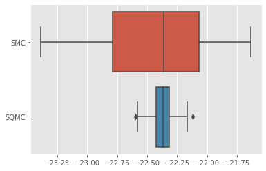
As expected, the variance of SQMC estimates is quite lower.

Command multiSMC makes it possible to run several particle filters, with varying options. Parallel execution is also possible, as explained in next tutorial.

Smoothing

So far, we have only considered filtering; let’s try smoothing, that is, approximating the distribution of the whole trajectory \(X_{0:T}\), given data \(Y_{0:T}=y_{0:T}\), for some fixed time horizon \(T=100\). In particular, we are going to sample smoothing trajectories from the output of the first particle filter we ran a few steps above.

smooth_trajectories = pf.hist.backward_sampling(10)
plt.figure()
plt.plot(smooth_trajectories);

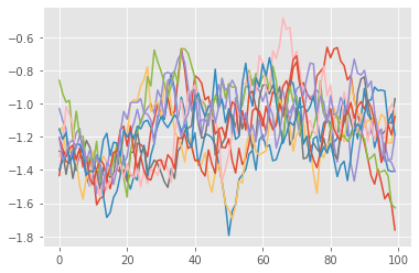
Here, we used the standard version of the FFBS (forward filtering, backward sampling) algorithm, which generates smoothing trajectories from the particle history (which we generated when running pf above). Other smoothing algorithms are available, see the next tutorial.

(Bayesian) Parameter estimation

Finally, we consider how to estimate the parameter \(\theta=(\alpha, \rho, \sigma)\) from a given data-set. First, we set up a prior as follows.

prior_dict = {'mu':dists.Normal(),
              'sigma': dists.Gamma(a=1., b=1.),
              'rho':dists.Beta(9., 1.)}
my_prior = dists.StructDist(prior_dict)

Again, the code above should be fairly readable: the prior for \(\mu\) is \(N(0,1)\), the one for \(\sigma\) is a Gamma(1,1) and so on. (As before, probability distributions are represented by objects defined in the distributions module.)

This may not be a sensible prior distribution; for instance it restricts \(\rho\) to \([0,1]\). However, this will suffice for our purposes. A popular way to simulate from the posterior distribution of the parameters of a state-space model is PMMH, a particular instance of the PMMC framework. Basically, this is a MCMC algorithm that runs at each iteration a particle filter so as to evaluate the likelihood.

%%capture
from particles import mcmc  # where the MCMC algorithms (PMMH, Particle Gibbs, etc) live
pmmh = mcmc.PMMH(ssm_cls=StochVol, prior=my_prior, data=data, Nx=50, niter = 1000)
pmmh.run()  # Warning: takes a few seconds

Again, the code above is hopefully readable: PMMH is run for 1000 iterations (niter), the particle filter run at each iteration have \(N_x=50\) particles, and so on. One point worth mentioning is that we pass as an argument the class StochVol. Again, remember that this class indeed represents the considered parametric class (as opposed to my_model, which was a stochastic volatility model, for certain fixed parameter values).

OK, we have waited long enough, let’s plot the results.

# plot the marginals
burnin = 100  # discard the 100 first iterations
for i, param in enumerate(prior_dict.keys()):
    plt.subplot(2, 2, i+1)
    sb.distplot(pmmh.chain.theta[param][burnin:], 40)
    plt.title(param)

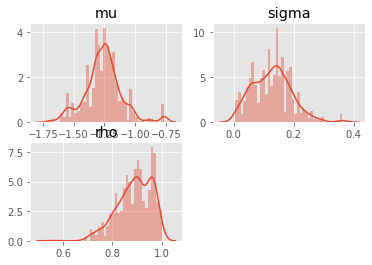
These results might not be very reliable, given that we used a fairly small number of MCMC iterations. If you are familiar with MCMC, you may wonder how the Metropolis proposal was set: by default, PMMH uses an adaptive Gaussian random walk proposal, such that the covariance matrix of the random step is iteratively adapted to the running simulation.

The library also implements SMC\(^2\), and Particle Gibbs, but that will be covered in the next tutorial.

The end

That’s all, folks! This very basic tutorial is over. If you crave for more, head to the other tutorials:

• Advanced tutorial for state-space models: covers the same topics as above (filtering, smoothing, parameter estimation for state-space models) but with more details.

• Tutorial on Bayesian estimation: covers PMCMC and SMC^2 algorithms that may be used to estimate the parameters of a state-space model.

• Tutorial on SMC samplers: a tutorial on how to run a SMC sampler (such as IBIS or tempering SMC) for a given static target distribution.

• How to define manually Feynman-Kac models: an advanced tutorial on how to define your own Feynman-Kac models.